How Depreciation Works

Everything the Fixed Assets module does with depreciation comes out of a single line of arithmetic applied once per fiscal period. There is no rate table, no method library and — this surprises people — no depreciation-rate field anywhere on the asset. Once you have that one line in your head, every other page in this folder becomes obvious: the depreciation run applies it, the addition and deduction document changes one of its inputs, the properties document changes another, and revaluation replaces it altogether.

So this page is the one to read first, and the one to come back to when a figure on a depreciation run does not look like the figure you expected.

Two Methods, and Only Two

Every asset carries an Asset Depreciation Method (طريقة إهلاك الأصل) on its master file, and it can hold one of exactly two values:

Method	Label	What it means
Straight Line	Straight Line / قسط ثابت	The system computes the periodic charge from the formula below. This is the default on every new asset.
Revaluation	Revaluation / إعادة تقييم	The system computes nothing. You state the asset's appraised value each time it is re-appraised, and the difference is booked as a gain or a loss.

There is no reducing balance, no sum-of-digits, no units-of-production and no declining-balance option — those methods are not implemented and no setting turns them on. If your accounting policy requires one of them, it has to be handled outside the module.

The method is chosen on the asset and cannot be swapped once the asset has any history behind it, so it is a decision made when the asset is created rather than an ongoing setting. It also decides which document may touch the asset: a straight-line asset is depreciated by the depreciation document and is refused by the revaluation document, and a revaluation-method asset is the mirror image — the depreciation run will not even collect it. Everything from here to the end of this page is about straight-line assets; revaluation has its own page.

One Formula

Here it is, in full:

instalment = (current value − salvage value) ÷ remaining life

where current value is the asset's carrying amount at that moment — cost, plus everything capitalised onto it, less everything deducted from it, less all depreciation charged so far.

The formula is not evaluated once when the asset is created and then repeated. It is re-derived from scratch every single period, from whatever the three inputs happen to be at that moment. That is the single most important thing to understand about this module, and the reason the rest of this folder works the way it does.

Take MCH-0007, Al-Waha Industries' CNC cutting machine, bought on 1 January 2026:

Cost	240,000
Salvage value	24,000
Useful life	60 months
Depreciation start date	1 January 2026

The first three periods look like this:

Period	Current value	Arithmetic	Instalment
Jan 2026	240,000	(240,000 − 24,000) ÷ 60	3,600
Feb 2026	236,400	(236,400 − 24,000) ÷ 59	3,600
Mar 2026	232,800	(232,800 − 24,000) ÷ 58	3,600

Both the numerator and the denominator shrink by exactly the right amount each period, so as long as nothing else happens to the asset the charge is flat — indistinguishable from classic straight line. The formula is doing more work than a fixed rate would, but on an undisturbed asset it produces the same answer.

The instalment is rounded to the number of decimal places the currency uses, so on a two-decimal currency you will see figures like 2,347.92 rather than long fractions.

Life Is Counted in Periods, Not Years

Useful Life (العمر الإفتراضي) and Remaining Life (العمر المتبقي) are counts of fiscal periods, held in months. MCH-0007's useful life of 60 means sixty monthly periods, not sixty years and not five entries.

Remaining life is reduced by exactly one every time a depreciation entry is committed for the asset. That is the whole mechanism — there is no schedule table, no end-date countdown and no rate to reconcile. The rate is implied: dividing by 60, then 59, then 58 is the rate.

Because the divisor is a count of periods, the module expects monthly fiscal periods, and every example in this documentation assumes a fiscal year of twelve monthly periods. Set the fiscal calendar up that way before the first asset is entered — it is one of the two decisions that are painful to revisit later.

The First Period Is a Full Period

There is no proration and no partial first period. An asset put into service on the 28th of a month is charged exactly the same instalment as one put into service on the 1st. MCH-0007 would have been charged 3,600 for January 2026 whether it was bought on 1 January or 31 January.

This is not an option you can switch; the formula contains no day count at all. What the system does instead is insist that the first depreciation of an asset falls in the fiscal period that contains its depreciation start date. If you want the machine to start depreciating in February, you move its depreciation start date into February — that is the only lever there is.

The trap that follows from this

Because the first run must land in the period containing the start date, an asset whose very first period was simply missed will not be picked up by any later run, and the run gives no reason — the asset just is not in the list. If you find an asset that never appears on a depreciation document, check its depreciation start date against the periods you have already run. Bridging the gap is what the prevent depreciation document is for.

The Schedule Corrects Itself

Because the instalment is re-derived every period, any change to the asset's value, salvage or remaining life simply changes the next instalment. Nothing is restated, no catch-up entry is ever created, and nothing needs to be recalculated by hand.

Follow MCH-0007 through its first year. Twelve runs at 3,600 leave it here at the end of December 2026:

Accumulated depreciation	12 × 3,600 = 43,200
Book value	240,000 − 43,200 = 196,800
Remaining life	48 periods

In January 2027 the machine gets a control-unit upgrade worth 30,000, capitalised through an addition and deduction document. The next depreciation run does not consult a schedule; it evaluates the formula again with the new numbers:

(196,800 + 30,000 − 24,000) ÷ 48 = 202,800 ÷ 48 = 4,225

The instalment moves from 3,600 to 4,225 and stays there. The machine's total cost is now 270,000, its end date is unchanged, and the extra 30,000 is spread over the periods that are left rather than over the periods that have already gone. The twelve entries of 2026 are untouched.

Exactly the same thing happens when a properties document shortens the remaining life, when a partial disposal takes part of the cost away, or when a deduction writes value off. One input changes; the next instalment reflects it; history stands.

When Depreciation Stops

Three things end an asset's depreciation, and all three do it by changing what the formula returns or what the run is willing to collect:

• Salvage value is reached. When the value left to depreciate falls to salvage or below, the committing run flips the asset's status to Depreciated (مهلك) and it stops being collected.
• Remaining life reaches zero. The instalment becomes zero and the status becomes Depreciated — or Not Depreciable if the asset was flagged as not depreciable.
• The asset is disposed of. A disposal takes the carrying amount to zero, sets remaining life to zero and moves the asset to Disposed.

That last one has a string attached, and it is worth knowing before you plan a disposal: the dependency runs both ways. A disposal reads the asset's posted balances rather than computing a catch-up instalment, so it refuses to commit while the asset's depreciation is behind — if a fiscal period has been left un-depreciated between the asset's last depreciation and the disposal, you have to run and process those periods first. See Disposing of an Asset.

Statuses are covered in full on Asset Statuses.

What the Run Needs Before It Will Touch an Asset

When you press Collect Assets on a depreciation document, an asset is offered only if all of the following are true. This list is the answer to almost every "why is my asset not on the list?" question:

• its status is Running — an asset still in its initial state, disposed, fully depreciated or flagged not depreciable is never collected;
• its method is Straight Line;
• its depreciation start date falls on or before the end of the chosen period;
• it has not been depreciated in this period already, and the period is the one immediately following its last depreciation period — the series has to be consecutive, with no skipped periods;
• no committed prevent depreciation document covers it for that period;
• the computed instalment is greater than zero.

The Asset's Value Timeline

Behind every asset is a dated timeline of value events. Each document that changes an asset — purchase, opening, depreciation, addition, deduction, revaluation, properties change, prevention, disposal — writes exactly one dated entry onto it, and the asset's current figures are the result of replaying that timeline in date order.

Two consequences matter in daily work:

1. Value date is load-bearing. A document cannot be inserted in front of an entry that already exists for the same asset; you will be told the asset already has a transaction on a later date in another document. Work forwards, not backwards.
2. Cancellations go newest-first. To undo a depreciation run for an asset that has been depreciated three times since, cancel the three later runs first. The same rule applies to every document in this folder.

You can read the result of that timeline on the asset's Statistics page, which is where accumulated depreciation, current value, remaining life and the current instalment are shown.

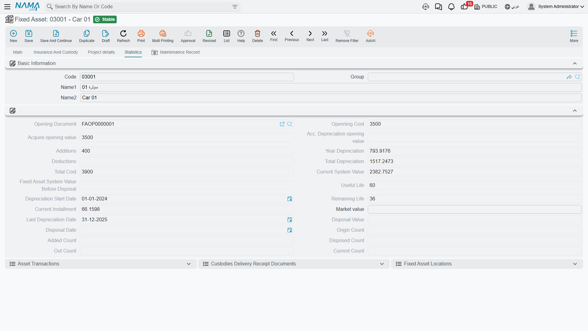
Nothing on that page is typed. Every figure on it is the arithmetic of this page, replayed over the documents that have touched the asset.